owslib is a Python package for client programming with OGC web service interface standards.
In this tutorial we’ll work with the four types of interfaces we’ve seen
so far: WMS, WFS, WCS and WPS. But there are other interfaces supported
by owslib that are of potential interest, namely the csw (Catalog
services), sos (Sensor Observation Services) and waterml (Water
Markup Language).
In [4]:
import owslib
owslib.__version__
Out[4]:
'0.16.0'
In [5]:
from owslib.wms import WebMapService
from owslib.wfs import WebFeatureService
from owslib.wcs import WebCoverageService
from owslib.wps import WebProcessingService
#
from owslib.csw import CatalogueServiceWeb
from owslib.sos import SensorObservationService
from owslib.waterml.wml11 import WaterML_1_1
from owslib.wmts import WebMapTileService
Web Mapping Service
We start by fetching a map using the WMS protocol. We first instantiate
a WebMapService object using the address of the NASA server, then
browse through its content.
In [ ]:
wms = WebMapService('https://neowms.sci.gsfc.nasa.gov/wms/wms')
print("Title: ", wms.identification.title)
print("Type: ", wms.identification.type)
print("Operations: ", [op.name for op in wms.operations])
print("GetMap options: ", wms.getOperationByName('GetMap').formatOptions)
wms.contents.keys()
The content is a dictionary holding metadata for each layer. We’ll
print some of the metadata’ title for a couple of layers to see what’s
in it.
In [5]:
for key in ['MOD14A1_M_FIRE', 'CERES_LWFLUX_M', 'MOD11C1_M_LSTDA', 'ICESAT_ELEV_G', 'MODAL2_M_CLD_WP', 'MOD_143D_RR']:
    print(wms.contents[key].title)
Active Fires (1 month - Terra/MODIS)
Outgoing Longwave Radiation (1 month)
Land Surface Temperature [Day] (1 month - Terra/MODIS)
Greenland / Antarctica Elevation
Cloud Water Content (1 month - Terra/MODIS)
True Color (1 day - Terra/MODIS Rapid Response)
We’ll select the true color Earth imagery from Terra/MODIS. Let’s check out some of its properties. We can also pretty print the full abstract with HTML.
In [6]:
from IPython.core.display import HTML

name = 'MOD_143D_RR'
layer = wms.contents[name]
print("Abstract: ", layer.abstract)
print("BBox: ", layer.boundingBoxWGS84)
print("CRS: ", layer.crsOptions)
print("Styles: ", layer.styles)
print("Timestamps: ", layer.timepositions)
HTML(layer.parent.abstract)
Abstract:  None
BBox:  (-180.0, -90.0, 180.0, 90.0)
CRS:  ['EPSG:4326']
Styles:  {}
Timestamps:  ['2006-09-01/2006-09-14/P1D', '2006-09-17/2006-10-10/P1D', '2006-10-12/2006-11-18/P1D', '2006-11-21/2007-03-01/P1D', '2007-03-03/2007-08-16/P1D', '2007-08-18', '2007-08-20/2007-09-11/P1D', '2007-09-15/2007-12-30/P1D', '2008-01-01/2008-01-24/P1D', '2008-01-27/2008-02-24/P1D', '2008-02-26/2008-03-18/P1D', '2008-03-20/2008-06-12/P1D', '2008-06-14', '2008-06-16/2008-07-12/P1D', '2008-07-14/2008-09-17/P1D', '2008-09-19', '2008-09-22/2008-10-17/P1D', '2008-10-19/2008-10-22/P1D', '2008-10-28/2008-12-02/P1D', '2008-12-04/2008-12-20/P1D', '2008-12-23/2008-12-30/P1D', '2009-01-01/2009-01-20/P1D', '2009-01-22/2009-04-19/P1D', '2009-04-23/2009-07-05/P1D', '2009-07-08/2009-12-30/P1D', '2010-01-01/2010-07-16/P1D', '2010-07-18/2010-12-07/P1D', '2010-12-09/2010-12-30/P1D', '2011-01-01/2011-01-25/P1D', '2011-01-27/2011-03-19/P1D', '2011-03-21/2011-07-23/P1D', '2011-07-27/2011-08-27/P1D', '2011-08-30/2011-12-13/P1D', '2011-12-15/2012-02-19/P1D', '2012-02-21/2013-12-01/P1D', '2013-12-04/2018-03-12/P1D', '2018-03-14/2018-05-16/P1D', '2018-05-18/2018-09-16/P1D']
Out[6]:
These images show the Earth's surface and clouds in true color, like a photograph. NASA uses satellites in space to gather images like these over the whole world every day. Scientists use these images to track changes on Earth's surface. Notice the shapes and patterns of the colors across the lands. Dark green areas show where there are many plants. Brown areas are where the satellite sensor sees more of the bare land surface because there are few plants. White areas are either snow or clouds. Where on Earth would you like to explore?
Getting the image data
Now let’s get the image ! The response we’re getting is a
ResponseWrapper object, we need to read its content to get the
actual bytes for the png file. To avoid writing the data to disk, we’ll
mimic a file object in memory using the io.BytesIO function.
In [7]:
response = wms.getmap(layers=[name,],
                 styles=['rgb'],
                 bbox=(-180, -90, 180, 90), # Left, bottom, right, top
                 format='image/png',
                 size=(600,600),
                 srs='EPSG:4326',
                 time='2018-09-16',
                 transparent=True)
response
Out[7]:
<owslib.util.ResponseWrapper at 0x7fbc78447f60>
In [8]:
import io
image = io.BytesIO(response.read())
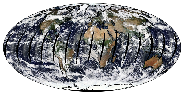
Plotting the image on a map
Using the cartopy library, we’ll overlay the image on a map of the
Earth.
In [9]:
import cartopy
import matplotlib.pyplot as plt
data = plt.imread(image)
In [10]:
fig = plt.figure(figsize=(8,6))
ax = fig.add_axes([0,0,1,1], projection=cartopy.crs.Mollweide())
ax.imshow(data, origin="upper", extent=(-180, 180, -90, 90),
          transform=cartopy.crs.PlateCarree())
ax.coastlines()
plt.show()
In [5]:
# Web Feature Services
#url = "http://geo.weather.gc.ca/geomet/wfs"
#wfs = WebFeatureService(url, version='1.1.0')
In [6]:
#print(wfs.contents.keys())
#name = 'ec-msc:HURRICANE_LINE'
In [7]:
#feature = wfs.getfeature(typename=name)
In [ ]:
… but the ECCC server only seems to output in GML format, which is a pain to convert to anything useful for plotting…