Spatial and temporal subsetting

A common task in climate data analysis is subsetting files over a region of interest. Global model simulations and observations cover the entire globe, while impact analyses are often concerned with a region. Instead of downloading the entire file on a local disk, it is often more practical to subset it on the server and only download the relevant part.

This can be done through two ways: interactive analysis using OPeNDAP, or a WPS request for a subsetter. Let’s start with the most direct approach with OPeNDAP. The PAVICS THREDDS server provides two links for each file, a link to the file itself which will download the file locally when accessed, and a dodsC link which supports the OPeNDAP protocol. We’ll use this link and simply pass it to our netCDF library, here xarray.

Subsetting with OPeNDAP

%matplotlib inline
import xarray as xr
import numpy as np
from matplotlib import pyplot as plt
# The dodsC link for the test file
dap = 'https://pavics.ouranos.ca/twitcher/ows/proxy/thredds/dodsC/'
ncfile = 'birdhouse/testdata/flyingpigeon/cmip5/tasmax_Amon_MPI-ESM-MR_rcp45_r1i1p1_200601-200612.nc'

# Here we open the file and subset it using xarray fonctionality, which communicates directly with
# the OPeNDAP server to retrieve only the data needed.
ds = xr.open_dataset(dap+ncfile)
tas = ds.tasmax
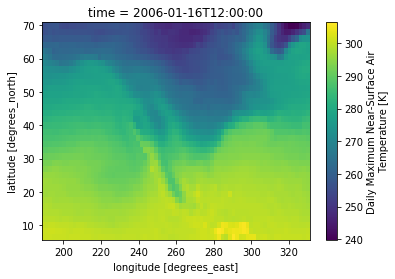
subtas = tas.sel(time=slice('2006-01-01', '2006-03-01'), lon=slice(188,330), lat=slice(6, 70))
subtas.isel(time=0).plot()
plt.show()

Subset processes with WPS and FlyingPigeon

PAVICS offers a number of subsetting processes through the FlyingPigeon WPS server: - subset_continents - subset_countries - subset_bbox - subset_wfs - subset

The subset_continents and subset_countries use a predefined list of polygons for the subsetting. The subset_bbox takes the geographical coordinates of the two opposite corner of a rectangle to define the subset region, while both subset_wfs and subset use a polygon defined on a remote geoserver, identified by a typename and a feature id. The only difference between those two is that subset also does temporal subsetting.

The first step to launch those services is to create a connexion to the WPS server using Birdy’s WPSClient.

from birdy import WPSClient
url = 'https://pavics.ouranos.ca/twitcher/ows/proxy/flyingpigeon/wps'
fp = WPSClient(url)

Now we’ll use fp.subset_continents, so let’s first check what arguments it expects and pass those to the function.

help(fp.subset_continents)

Help on method subset_continents in module birdy.client.base:

subset_continents(region='Africa', mosaic=None, resource=None) method of birdy.client.base.WPSClient instance
    Return the data whose grid cells intersect the selected continents for each input dataset.

    Parameters
    ----------
    region : {'Africa', 'Asia', 'Australia', 'North America', 'Oceania', 'South America', 'Antarctica', 'Europe'}string
        Continent name.
    mosaic : boolean
        If True, selected regions will be merged into a single geometry.
    resource : ComplexData:mimetype:`application/x-netcdf`, :mimetype:`application/x-tar`, :mimetype:`application/zip`
        NetCDF Files or archive (tar/zip) containing netCDF files.

    Returns
    -------
    output : ComplexData:mimetype:`application/x-tar`
        Tar archive of the subsetted netCDF files.
    ncout : ComplexData:mimetype:`application/x-netcdf`
        NetCDF file with subset for one dataset.
    output_log : ComplexData:mimetype:`text/plain`
        Collected logs during process run.

thredds = 'https://pavics.ouranos.ca/twitcher/ows/proxy/thredds/fileServer/'
ncfile = 'birdhouse/testdata/flyingpigeon/cmip5/tasmax_Amon_MPI-ESM-MR_rcp45_r1i1p1_200601-200612.nc'
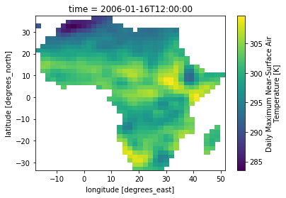
resp = fp.subset_continents(resource=thredds+ncfile, region='Africa')

The response we’re getting can either include the data itself or a reference to the data. Using the get method of the response object, we’ll get what was included in the response. If the response holds only a reference (link) to the output, we can retrieve it using the get(as_obj=True) method. Birdy will then inspect the file format of each output and try to find the appropriate way to open the file and return a Python object. A warning is issued if no converter is found, in which case the original reference is returned.

resp.get()
tar_out, nc_out, log = resp.get(asobj=True)

/home/david/src/birdy/birdy/client/outputs.py:65: UserWarning: No converter was found for mime type: application/x-tar
  warnings.warn(UserWarning("No converter was found for mime type: {}".format(output.mimeType)))

Next, we’ll open the netCDF dataset using xarray and plot the result. Note that since nc_out is an already opened netcdf4.Dataset, we’re using the xr.backends.NetCDF4DataStore function to open the dataset.

import xarray as xr
ds = xr.open_dataset(xr.backends.NetCDF4DataStore(nc_out))
ds.tasmax.isel(time=0).plot()

<matplotlib.collections.QuadMesh at 0x7fd774d672b0>